The mistakes
What I got wrong
Four things I published that turned out to be wrong. Two bugs that had been quietly ruining measurements. An effect I had pointing the wrong way, and a phase spent optimizing the wrong resource. Eight predictions I wrote down in advance and lost, four of them the headline of their write-up, and one correction that went too far and had to be walked back.
The big one
A setting that was 48 times too large
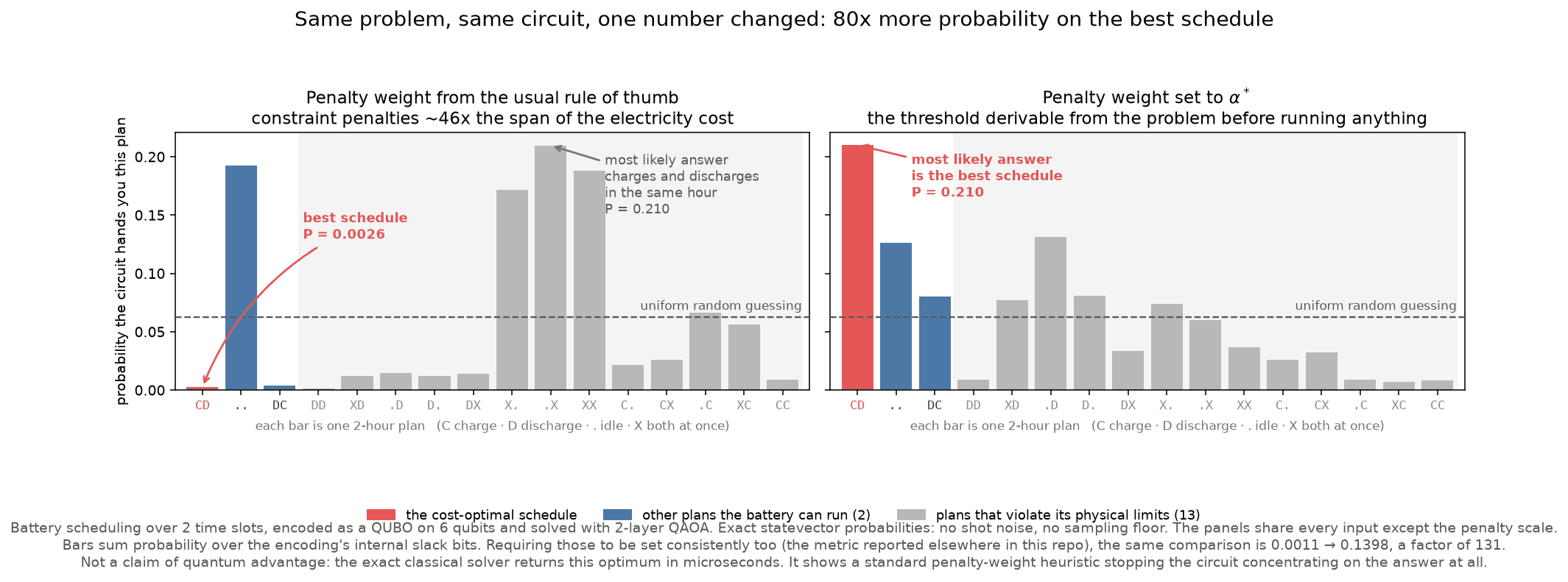
The circuit does two things at once: obey the battery's limits, and among the plans that do, find the cheapest. I set the penalty for breaking a rule 48 times larger than the whole spread between the cheapest and most expensive legal plan, which meant the machine was paid well for finding a legal plan and almost nothing for finding a cheap one.
Fixing that one number, with the circuit and the tuning untouched, improved how often it lands on the best plan by a factor of several hundred. The right value can be worked out from the problem in advance rather than tuned by hand.
Take a two-hour day, where there are sixteen possible plans, and ask the circuit how likely it is to hand you each one. At the setting I had been using, the plan it returns most often charges and discharges in the same hour, which no battery can do. The cheapest legal plan comes up 80 times less often than it does once the setting is fixed.
I had been showing a chart of how the quantum method scaled, every point of which was measured through the bad setting. On that chart the advantage shrank as problems grew, and several points sat below random guessing, meaning the circuit was doing worse than nothing.
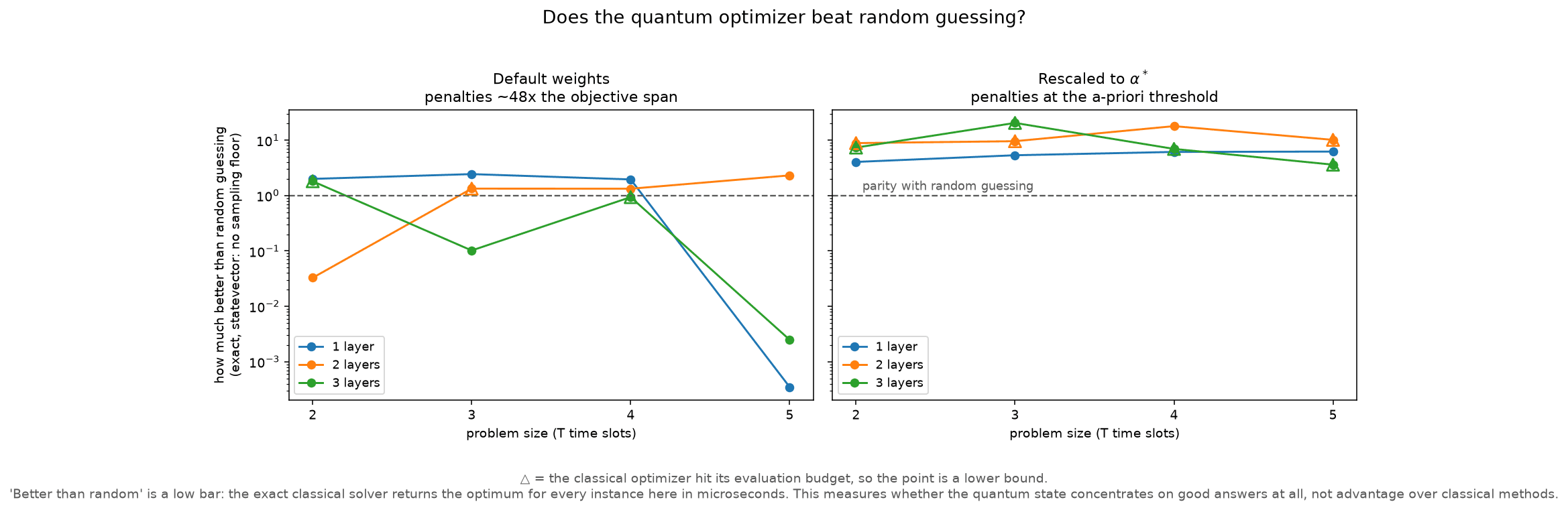
Re-running it moved the same measurements to 4 to 20 times better than chance at every size, with no decline as the problem grows, and turned finding the exact best plan at 14 qubits from something that happened twice in nine tries into something that happened eight times in nine.
One thing that chart is not claiming. Beating random guessing is a low bar here, because the ordinary classical solver returns the exact best plan for every one of these problems in microseconds. This measures whether the quantum state gathers around good answers at all, which is a different and much smaller question than beating a classical computer.
I had been reading that chart as something I had learned about quantum computing. Most of it was something I had learned about my own settings.
The other end of the chart
Zeros, a ceiling, and a tool that never worked
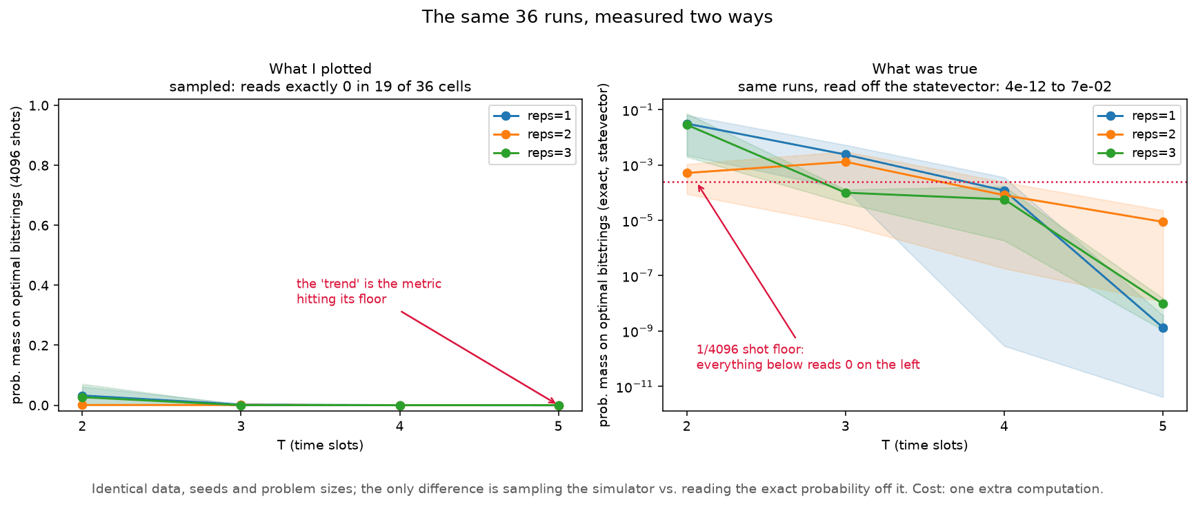
The old chart had a second problem, at the opposite end from the weight. Because it read the answer by sampling 4,096 times, anything rarer than one in 4,096 came back as a flat zero, and nineteen of its thirty-six measurements did. The declining trend I was describing was not the quantum method getting worse but my measurement hitting its own floor.
The fix cost one extra calculation, which reads the exact probability off the simulator instead of sampling it. With the same runs, the same seeds and the same problem sizes, the numbers that had read zero turned out to span 4e-12 to 7e-02.
While checking the corrected numbers I looked at how much tuning effort the runs had actually used. It came back at exactly the maximum I had allowed. Because a number sitting on its own limit measures the limit, not the thing, the figures from that sweep are floors rather than final answers, and the pages that quote them say so.
The tool computing the measurement had never worked above the smallest problem size. It builds something that doubles with every qubit, so it ran out of memory partway through. From outside that looks like a long job crashing rather than a broken instrument, which is why it went unnoticed.
Rewriting that one calculation took it from failing at 14 qubits to finishing 22 in about five seconds. It now checks itself against the old method before the study spends anything.
And then I over-corrected
Finding an error is not the same as knowing what it broke
Because an earlier conclusion rested on runs that had been sitting on the cap, I wrote that it was not supported. That was an overreach, which took 120 more runs to find out. The budget study has the runs.
The first half of what I had said was right. The budget was binding, since the original runs hit their limit on ten seeds out of ten. Lifting it twenty-five times did help, by a margin clear enough to measure.
It just did not help enough, because the gap the result had to close was about three times larger than everything the cap had been hiding. So the conclusion survived, although the measurement under it moved, because the move was not enough to change anything.
The extra budget went unused. Given twenty-five times the allowance, the optimizer spent 38% of it and stopped, so the limit was no longer binding at all. Whatever holds it back is something else.
The one run out of the 120 that did clear the bar came from the arm with the smallest budget, not the largest. If budget had been the problem, the well-funded runs would have cleared and the starved one would not. That is what a lucky start looks like rather than a resource limit.
A measurement stuck against its own limit tells you the number is imprecise, but not that it is pointing the wrong way. The only way to find out which is to raise the limit and look.
A test I failed
The instance I named first
Before putting a circuit on real hardware I wrote down what would justify it: a specific version of the problem, named in advance, and a bar the simulation had to clear. It did not clear. Twelve combinations of tuning strategy and setting, some with ten times the computing budget of the others, all failed, with the best coming out just under, at 0.075 against a required 0.078.
Several of those same strategies clear the bar on two other versions of the problem, one of them ten times out of ten. The version I named first is the hardest of the three. Because switching to one of the others after seeing that would answer a question I had not asked, the circuit did not run.
The question is still open, but not for lack of computing budget, because the verdict stood when I re-ran the study with the caps lifted. A deeper sweep later placed the obstacle in the rule that picks which tuning to trust, and a selection rule that fixes the pick has since been measured.
A model I kept trusting
Three misses in the same direction
My noise model is simple: every delicate two-qubit operation has some chance of scrambling the state, so a circuit's output should degrade at a fixed rate compounded over its operation count. Fitted to the July hardware run, that rate came out at about 1.32% per operation. The model has now made three predictions, and missed all three, every time predicting more damage than the machine delivered.
The third miss was pre-registered. On August 25 I predicted that one and two circuit layers would tie on hardware, because the deeper circuit's noise-free advantage of 1.93 times would be exactly eaten by 2.4 times the operations. The deeper circuit won by 4.7 times the threshold, then won again the next day when the identical circuits ran in a fresh calibration window. The first run's explanation for the win, that both depths lose the same fraction of their ideal answer, did not survive the replication, and the write-up withdraws it in place rather than deleting it.
The part I got wrong sat in my own files. The first two misses were already written up, each in its own document that said “the model failed here” and moved on, so no single document was responsible for the sequence, and I staked a third prediction on the model anyway. Three misses sharing a direction is a bias whose direction shows long before its size is understood. The repository now records the count where the rate is introduced, and no forward prediction leans on the model.
The wrong thing to count
I spent a phase optimizing the resource that was not the limit
Quantum computers are advertised by their qubit count, so that is what I worked on. A phase of this project went into the encoding that strips out the bookkeeping bits, which takes 22 qubits down to 12 on a six-hour problem and 117 down to 52 on a full day. When I then looked at data from a run I had already done, the qubit count explained nothing about how badly the machine mangled the answer.
What explains it is the number of two-qubit gates. Because every one of those is a physical operation with an error rate, and the errors compound, a gate costs something each time it runs, while a qubit sitting idle costs comparatively little.
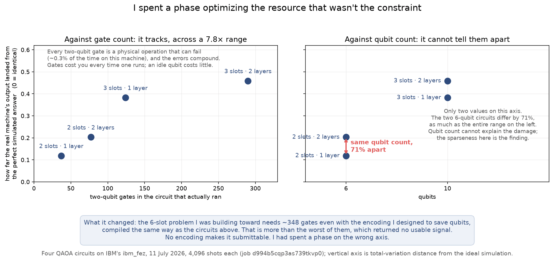
The encoding fits the problem on a smaller machine and loses none of the money. What it does not do is fix the noise, which I had been assuming it would.
The six-hour problem I was building toward needs 348 gates even with the smaller encoding, against 290 for the worst circuit in the run, which came back with almost no usable signal. No encoding makes that problem submittable. The run that shows this had already happened before the phase started.
A prediction I wrote down and lost
I had the shape of the answer backwards
Tuning the circuit starts from a random guess and walks downhill. Run it forty times and count how many different places it comes to rest. One place means the tuning is repeatable, while nineteen means the answer depends on where you started.
The setting I had derived, the one that fixed the 48 times error above, is 0.0209. Before running anything I wrote down what I expected, which was that tuning would be most repeatable at 0.0209 and less repeatable on either side of it, a valley with 0.0209 at the bottom. I also wrote down what would count as being wrong.
There is no low side. Tuning lands in the same place every time at 0.0209 and at every setting below it. Above it, repeatability falls apart quickly: two places at 0.030, three at 0.060, and nineteen at the setting I had been using before.
Repeatable is not the same as right. Below 0.010 the penalty is too weak to rule out plans the battery cannot actually run, so the tuning converges onto one of those, every time. At 0.003 it looks better than 0.0209 by the usual measure, although it is landing reliably on a plan that is not a schedule.
So the useful result is not the one I predicted. 0.0209 is not the middle of a safe range with room on both sides but the top of one. Going 1.4 times above the top of the range that is both correct and repeatable, which runs from 0.010 to 0.021, doubles the number of places the tuning can land.
This ran on a simulator and on exact arithmetic, with no time on a real machine. The plan and the result are separate documents, and the write-up states the falsification criterion it was measured against.
A second prediction, also lost
The answer exists and my rule cannot find it
The study above ran on the shallow version of the circuit. The deeper version is where the project's open question lives, which is whether any tuning can put five times more probability on the right answer than guessing would. I wrote down two predictions and ran the same kind of sweep there. 400 tunings, simulator and exact arithmetic only, no time on a real machine, the plan committed before the run.
The first prediction held. The deeper circuit's tuning is not repeatable anywhere, with at least eleven resting places at every setting, where the shallow version had exactly one at 0.0209 and below.
The second lost. Although I predicted no tuning would reach the five-times bar, one of the forty did.
Losing it is the useful part. A tuning has to be picked by proxy, the circuit's own energy score, because that is what a real machine can measure without already knowing the answer. Across the forty tunings the proxy tracks the thing I want closely through the bulk and points wrong at the top, where it selects a tuning 3.4 percent short of the bar rather than the one above it. More tries would not change the pick, because the winner does not have the best energy score. So the bar is reachable on this problem, and what falls short is the rule for choosing.
The rule that can find it turned out to be simple: keep the tuning that puts the most probability on plans the battery can run. I then ran three registered studies. In every sound, repeatable setting they tested, five fresh versions of the problem and four sizes, that pick was the best one available, and it clears the bar on both hard versions where the energy score misses. The limits travel with it, since only two of the six versions swept are hard enough to tell the rules apart and every size tested is still small enough to check exactly.
The write-up and the registered plan are separate documents, and the sweep refuses to run if the plan has been edited since it was committed. The replication follows the same discipline.
Backwards, not just imprecise
I had a whole effect pointing the wrong way
I said two things about the battery's savings for months. That the model assumed a battery losing nothing, so the real figure was lower. And that the model assumed power sells back at the price it was bought for, which real utilities do not pay, so the real figure was lower again. Both assumptions push the same way, I wrote, so every saving was a ceiling and every payback a floor.
The first half was right. A battery losing a tenth of what it stores saves $404.28 a year rather than $455.72, and payback at $11,500 goes from 25.2 years to 28.4. The gap is about a ninth, which I had called a ceiling without measuring.
The second half was backwards. A worse export credit makes the battery more valuable, not less. When the credit drops from full retail to a tenth of retail, the battery goes from $404.28 to $486.94 a year, and payback at $11,500 comes down from 28.4 years to 23.6.
What I had reasoned about was the discharge. If a utility pays little for exported power, a discharge that would have been exported earns little, so the battery earns less. That is true, although it is the smaller half. The larger half is power the house would otherwise have dumped onto the grid for almost nothing, which when stored instead displaces a kWh bought at retail. The worse the credit, the bigger that gap, and the more a battery is worth. Solar moves the other way over the same range, losing about 40%, which is why the two are reported separately and never added together.
The conclusion did not change. Payback at $11,500 used to be “at least 25 years, and worse once these assumptions are dropped.” It is now between 23.6 and 28.4 years for every value of both, against a 10-year warranty. Arbitrage does not pay for the hardware either way.
There is one row where it mattered. A $5,000 install with the faster battery used to pay back in 8.8 years, comfortably inside the warranty. It is 9.9 years, which clears by six weeks.
Retractions
Four claims I had to take back
Each of these was published before it was checked. The repository keeps every one where it was made, marked wrong.
- I blamed a difference between two circuits on the number of qubits, which my own earlier data does not support.
- I argued the machine could not have drifted between runs, using a comparison that was never valid. Drift is real, and worth 43% of that difference.
- I said the variation between runs was larger than the machine's own wobble within a run, although the two are too close to tell apart with the data I have.
- My first error bars used a method that added noise the measurement does not contain, which made my own result look weaker than it was.
Fixing that last one moved the lower bound eightfold.
One more
A second test in the same plan asked how much the machine varies within one job. I had written it as needing a spread “comparable to or larger than” the effect, never said what comparable meant, and then picked a number after seeing the data.
Fixing the wording would not have saved it either, because the test never had the power to answer the question. A spread estimated from a single pair of runs carries about 76% uncertainty, so it straddles any sensible threshold. Re-run later with ten repeats, it came back undecided rather than wrong.
Each of these is written up where it happened, and the repository collects them in LESSONS.md, which reads on its own and carries the numbers this page leaves out.
Keep reading